43 excel xy chart labels

› charts › quadrant-templateHow to Create a Quadrant Chart in Excel – Automate Excel Building the chart from scratch ensures that nothing gets lost along the way. Click on any empty cell. Switch to the Insert tab. Click the “Insert Scatter (X, Y) or Bubble Chart.” Choose “Scatter.” Step #2: Add the values to the chart. Once the empty chart appears, add the values from the table with your actual data. Chart.Axes method (Excel) | Microsoft Docs This example adds an axis label to the category axis on Chart1. VB Copy With Charts ("Chart1").Axes (xlCategory) .HasTitle = True .AxisTitle.Text = "July Sales" End With This example turns off major gridlines for the category axis on Chart1. VB Copy Charts ("Chart1").Axes (xlCategory).HasMajorGridlines = False

Excel Chart VBA - 33 Examples For Mastering Charts in ... - Analysistabs Charts.Add End Sub 3. Adding New Chart for Selected Data using Charts.Add Method : In Existing Sheet using Excel VBA We can use the Charts.Add method to create a chart in existing worksheet. We can specify the position and location as shown below. This will create a new chart in a specific worksheet.

Excel xy chart labels

How To Show Two Sets of Data on One Graph in Excel Below are steps you can use to help add two sets of data to a graph in Excel: 1. Enter data in the Excel spreadsheet you want on the graph. To create a graph with data on it in Excel, the data has to be represented in the spreadsheet. For multiple variables that you want to see plotted on the same graph, entering the values into different ... How to make a quadrant chart using Excel | Basic Excel Tutorial It is done to ensure all the values and variables are included. To create it, follow these steps 1. Click on an empty cell 2. Go to the Insert tab 3. On the Charts dialog box, select the X Y (Scatter) to display all types of charts. 5. Click Scatter. An empty chart will appear on your worksheet. Add values to the chart. 1. Label line chart series - Get Digital Help To label each line we need a cell range with the same size as the chart source data. Simply copy the chart source data range and paste it to your worksheet, then delete all data. All cells are now empty. Copy categories (Regions in this example) and paste to the last column (2018). Those correspond to the last data points in each series.

Excel xy chart labels. peltiertech.com › multiple-time-series-excel-chartMultiple Time Series in an Excel Chart - Peltier Tech Aug 12, 2016 · Displaying Multiple Time Series in A Line-XY Combo Chart. Now for a short trip down Memory Lane. In Excel 2003 and earlier, you could plot an XY series along a Line chart axis, and it worked really well. The line chart axis gave you the nice axis, and the XY data provided multiple time series without any gyrations. How to change dot label(when I hover mouse on that dot) of - Microsoft ... 1. Can I edit the text when I hover mouse on dot of scatter plot (chart) 2. Can I use url to redirect to different site. 3. Can I use display image if I hover mouse on the dot. Please confirm me.. I really need to know.. If do I have use macro for this.. can anyone help me. Data is like this: Name X Y. ABC 2 4. XYZ 5 8 Make Excel Chart Gridlines Square - Peltier Tech sub squarexygridofselectedcharts () if not activechart is nothing then squarexychartgrid activechart, true, true elseif typename (selection) = "drawingobjects" then dim shp as shape for each shp in selection.shaperange if shp.haschart then squarexychartgrid shp.chart, true, true end if next else msgbox "select one or more charts and … How to Add Labels to Scatterplot Points in Excel - Statology Step 3: Add Labels to Points. Next, click anywhere on the chart until a green plus (+) sign appears in the top right corner. Then click Data Labels, then click More Options…. In the Format Data Labels window that appears on the right of the screen, uncheck the box next to Y Value and check the box next to Value From Cells.

support.microsoft.com › en-us › topicHow to use a macro to add labels to data points in an xy ... The labels and values must be laid out in exactly the format described in this article. (The upper-left cell does not have to be cell A1.) To attach text labels to data points in an xy (scatter) chart, follow these steps: On the worksheet that contains the sample data, select the cell range B1:C6. Quickly creating a x-y scatter chart with straight lines and markers ... Select the range. Insert a scatter chart with lines and markers. If it looks wrong, click anywhere in the chart. On the Chart Design tab of the ribbon, click Switch Row/Column. Here is an example. First, the scatter chart as created by Excel: Next, the result of clicking Switch Row/Column: How to Add a Vertical Line to Charts in Excel - Statology Suppose we would like to create a line chart using the following dataset in Excel: Step 2: Add Data for Vertical Line. Now suppose we would like to add a vertical line located at x = 6 on the plot. We can add in the following artificial (x, y) coordinates to the dataset: Step 3: Create Line Chart with Vertical Line Excel Bubble Chart Timeline Template - Vertex42.com A Bubble Chart in Excel is a relatively new type of XY Chart that uses a 3rd value (besides the X and Y coordinates) to define the size of the Bubble. Beginning with Excel 2013, the data labels for an XY or Bubble Chart series can be defined by simply selecting a range of cells that contain the labels (whereas originally you had to link ...

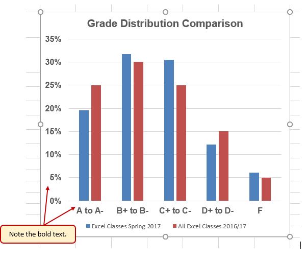
chandoo.org › wp › change-data-labels-in-chartsHow to Change Excel Chart Data Labels to Custom Values? May 05, 2010 · First add data labels to the chart (Layout Ribbon > Data Labels) Define the new data label values in a bunch of cells, like this: Now, click on any data label. This will select “all” data labels. Now click once again. At this point excel will select only one data label. How to Change the X-Axis in Excel - Alphr Follow the instructions to change the text-based X-axis intervals: Open the Excel file and select your graph. Now, right-click on the Horizontal Axis and choose Format Axis… from the menu. Select... How to Apply a Filter to a Chart in Microsoft Excel - How-To Geek Select the chart and you'll see buttons display to the right. Click the Chart Filters button (funnel icon). When the filter box opens, select the Values tab at the top. You can then expand and filter by Series, Categories, or both. Simply check the options you want to view on the chart, then click "Apply." XY Chart Labeler (free) download Windows version A very commonly requested Excel feature is the ability to add labels to XY chart data points. The XY Chart Labeler adds this feature to Excel. The XY Chart Labeler provides the following options: - Add XY Chart Labels - Adds labels to the points on your XY Chart data series based on any range of cells in the workbook.

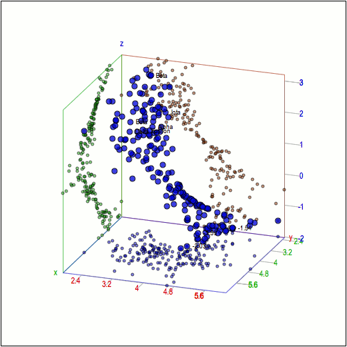
3d scatter plot for MS Excel

Scatter Graph from Pivot table . . . - Microsoft Tech Community I have managed to create a pivot chart, but is there a way to take those fields and display them ... Labels: Labels: Charting ... A pivot chart cannot be an XY Scatter chart. But see Excel Scatter Pivot Chart for a workaround. 0 Likes . Reply. mtm426 . replied to Hans Vogelaar ‎Dec 29 2021 08:59 PM. Mark as New; Bookmark;

30 Label X And Y Axis In Excel - Best Labeling Ideas

peltiertech.com › add-horizontal-line-to-excel-chartAdd a Horizontal Line to an Excel Chart - Peltier Tech Sep 11, 2018 · The examples below show how to make combination charts, where an XY-Scatter-type series is added as a horizontal line to another type of chart. Add a Horizontal Line to an XY Scatter Chart. An XY Scatter chart is the easiest case. Here is a simple XY chart.

Create a Line Chart in Excel - Easy Excel Tutorial

› charts › dynamic-chart-dataCreate Dynamic Chart Data Labels with Slicers - Excel Campus Feb 10, 2016 · Typically a chart will display data labels based on the underlying source data for the chart. In Excel 2013 a new feature called “Value from Cells” was introduced. This feature allows us to specify the a range that we want to use for the labels. Since our data labels will change between a currency ($) and percentage (%) formats, we need a ...

Bar-Line (XY) Combination Chart in Excel - Peltier Tech Blog

How to Change the Y Axis in Excel - Alphr No matter what values and text you want to show on the vertical axis (Y-axis), here's how to do it. In your chart, click the "Y axis" that you want to change. It will show a border to ...

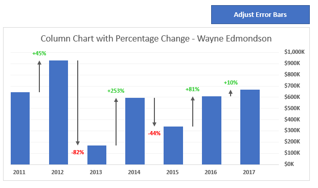
Column Chart That Displays Percentage Change or Variance - Excel Campus

How to add leader lines to a chart in Excel? - tutorialspoint.com After you have added your data labels, you will need to pick the data to get there. Step 6 Click the label that you want to format, and then click the Chart Elements button followed by the Data Labels button followed by the More Options button. Step 7

Advanced Graphs Using Excel : Radar plot

How to make a scatter plot in Excel - Ablebits.com Select the Value From Cells box, and then select the range from which you want to pull data labels (B2:B6 in our case). If you'd like to display only the names, clear the X Value and/or Y Value box to remove the numeric values from the labels. Specify the labels position, Above data points in our example. That's it!

Share :