41 display data labels in excel
Display every "n" th data label in graphs - Microsoft Community With this tool you can assign a range of cells to be the labels for chart series, instead of the Excel defaults. Using a formula, you can have a text show up in every nth cell and then use that range with the XY Chart Labeler to display as the series label. The tool can be downloaded here: Displaying data from excel to labels/buttons I have a large spreadsheet with 4,000 rows and four columns and I'd like to be able to display the information from individual cells in the spreadsheet as text on labels and buttons in a VB form. I'd rather not have to convert the spreadsheet into a SQL database if I don't have to. I messed ... · Hi Shemtheo, You can use excel automation to implement ...
How to use data labels in a chart - YouTube Excel charts have a flexible system to display values called "data labels". Data labels are a classic example a "simple" Excel feature with a huge range of o...
Display data labels in excel
Office: Display Data Labels in a Pie Chart - Tech-Recipes 1. Launch PowerPoint, and open the document that you want to edit. 2. If you have not inserted a chart yet, go to the Insert tab on the ribbon, and click the Chart option. 3. In the Chart window, choose the Pie chart option from the list on the left. Next, choose the type of pie chart you want on the right side. 4. Chart: Display alternative values as Data Labels or Data Callouts - MrExcel Joined. Aug 11, 2017. Messages. 1. Aug 11, 2017. #1. Below is my excel chart. I would like to add a "data labels" or "data callouts". As you can see the line is displaying the data from Actual X and Y, but I want to display the DEV values on this line. excel - How to not display labels in pie chart that are 0% - Stack Overflow Generate a new column with the following formula: =IF (B2=0,"",A2) Then right click on the labels and choose "Format Data Labels". Check "Value From Cells", choosing the column with the formula and percentage of the Label Options. Under Label Options -> Number -> Category, choose "Custom". Under Format Code, enter the following:
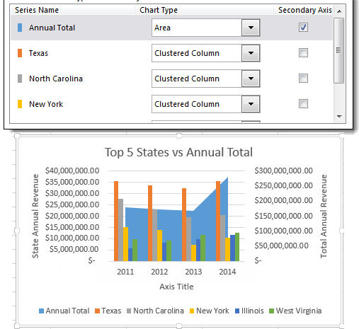
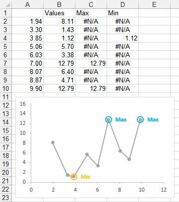
Display data labels in excel. 3D maps excel 2016 add data labels Re: 3D maps excel 2016 add data labels I don't think there are data labels equivalent to that in a standard chart. The bars do have a detailed tool tip but that required the map to be interactive and not a snapped picture. You could add annotation to each point. Select a stack and right click to Add annotation. Cheers Andy Excel tutorial: How to use data labels Generally, the easiest way to show data labels to use the chart elements menu. When you check the box, you'll see data labels appear in the chart. If you have more than one data series, you can select a series first, then turn on data labels for that series only. You can even select a single bar, and show just one data label. How to format axis labels as thousands/millions in Excel? Right click at the axis you want to format its labels as thousands/millions, select Format Axisin the context menu. 2. In the Format Axisdialog/pane, click Number tab, then in theCategorylist box, select Custom, and type[>999999] #,,"M";#,"K"into Format Codetext box, and click Addbutton to add it toTypelist. See screenshot: 3. Excel tutorial: Dynamic min and max data labels To make the formula easy to read and enter, I'll name the sales numbers "amounts". The formula I need is: =IF (C5=MAX (amounts), C5,"") When I copy this formula down the column, only the maximum value is returned. And back in the chart, we now have a data label that shows maximum value. Now I need to extend the formula to handle the minimum value.
How to Customize Your Excel Pivot Chart Data Labels - dummies The Data Labels command on the Design tab's Add Chart Element menu in Excel allows you to label data markers with values from your pivot table. When you click the command button, Excel displays a menu with commands corresponding to locations for the data labels: None, Center, Left, Right, Above, and Below. None signifies that no data labels ... Displaying Large Numbers in K (thousands) or M (millions) in Excel Simply select the number cell, or a range of numbers that you would like to convert into K or M. Right Click, and choose Custom Formatting. You can also choose Number Formatting from the Home Ribbon, or simply press the shortcut [Ctrl] + 1. Go to Custom, and key in 0, "K" in the place where it says General. Now close the Format Cells popup ... Change the format of data labels in a chart To get there, after adding your data labels, select the data label to format, and then click Chart Elements > Data Labels > More Options. To go to the appropriate area, click one of the four icons ( Fill & Line, Effects, Size & Properties ( Layout & Properties in Outlook or Word), or Label Options) shown here. How to add data labels from different column in an Excel chart? Right click the data series in the chart, and select Add Data Labels > Add Data Labels from the context menu to add data labels. 2. Click any data label to select all data labels, and then click the specified data label to select it only in the chart. 3.
10 spiffy new ways to show data with Excel | Computerworld In Cell C2 enter "=A2" and format the cell as General. You'll see a number like 43205, which is Excel's time/date code needed for the chart layout. Finally, in C3 enter "=C2+D2", then copy and ... VBA Excel: ElementDataLabelCallout display Data - Stack Overflow This answer is not useful. Show activity on this post. I have found the solution myself with recording a Macro its somewhat like this: ActiveSheet.ChartObjects ("Chart 1").Activate ActiveChart.FullSeriesCollection (1).DataLabels.Select Selection.ShowPercentage = False Selection.ShowValue = True. Share. Add a Data Callout Label to Charts in Excel 2013 In the upper right corner, next to your chart, click the Chart Elements button (plus sign), and then click Data Labels. A right pointing arrow will appear, click on this arrow to view the submenu. Select Data Callout. Once the Data Callout Labels have been added, you can re-position them by clicking on their borders and dragging to a new position. Excel charts: how to move data labels to legend You can't do that, but you can show a data table below the chart instead of data labels: Click anywhere on the chart. On the Design tab of the ribbon (under Chart Tools), in the Chart Layouts group, click Add Chart Element > Data Table > With Legend Keys (or No Legend Keys if you prefer)
Working with Multiple Data Series in Excel | Pryor Learning Solutions
Display data on user form - OzGrid Free Excel/VBA Help Forum 10. Jun 13th 2004. #5. Thanks Dave, Code is running well, instead of using combo box i changed it to textbox so i can enter data data manually. clicking a command button will search and display all data related to that on a labels. i used FIND but i find it confusing: can you enlighten me with this code. A1 E12345.
Highlight Minimum and Maximum in an Excel Chart - Peltier Tech
Outside End Data Label for a Column Chart (Microsoft Excel) 2. When Rod tries to add data labels to a column chart (Chart Design | Add Chart Element [in the Chart Layouts group] | Data Labels in newer versions of Excel or Chart Tools | Layout | Data Labels in older versions of Excel) the options displayed are None, Center, Inside End, and Inside Base. The option he wants is Outside End.

Pie Chart - PK: An Excel Expert
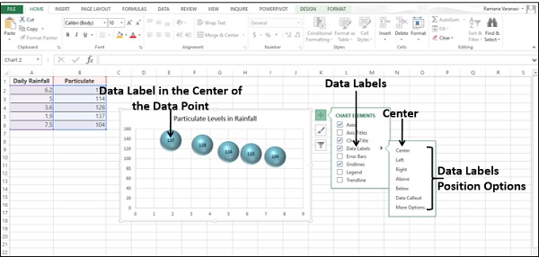
How to add or move data labels in Excel chart? - ExtendOffice 2. Then click the Chart Elements, and check Data Labels, then you can click the arrow to choose an option about the data labels in the sub menu. See screenshot: In Excel 2010 or 2007. 1. click on the chart to show the Layout tab in the Chart Tools group. See screenshot: 2. Then click Data Labels, and select one type of data labels as you need ...

GANTT Procedure
Custom Chart Data Labels In Excel With Formulas Follow the steps below to create the custom data labels. Select the chart label you want to change. In the formula-bar hit = (equals), select the cell reference containing your chart label's data. In this case, the first label is in cell E2. Finally, repeat for all your chart laebls.
Excel Dashboards - Краткое руководство - CoderLessons.com
Add or remove data labels in a chart - support.microsoft.com Right-click the data series or data label to display more data for, and then click Format Data Labels. Click Label Options and under Label Contains, select the Values From Cells checkbox. When the Data Label Range dialog box appears, go back to the spreadsheet and select the range for which you want the cell values to display as data labels.
November 2018
Format Data Labels in Excel- Instructions - TeachUcomp, Inc. Then select the "Format Data Labels…" command from the pop-up menu that appears to format data labels in Excel. Using either method then displays the "Format Data Labels" task pane at the right side of the screen. Set the values and positioning of the data labels in the "Label Options" category, which is shown by default.
Excel - Line Chart
Formatting Data Label and Hover Text in Your Chart - Domo In Chart Properties , click Data Label Settings. (Optional) Enter the desired text in the Text field. You can insert macros here by clicking the "+" button and selecting the desired macro. For more information about macros, see Data label macros. (Optional) Set the other options in Data Label Settings as desired.
Post a Comment for "41 display data labels in excel"