40 data labels excel pie chart
Solved: Pie Chart Not Showing all Data Labels - Power BI PASS Data Community Summit 2022 returns as a hybrid conference. You'll get to hear from industry-leading experts, make connections, and discover cutting edge data platform products and services. Learn More! How to Create and Format a Pie Chart in Excel - Lifewire Select the plot area of the pie chart. Select a slice of the pie chart to surround the slice with small blue highlight dots. Drag the slice away from the pie chart to explode it. To reposition a data label, select the data label to select all data labels. Select the data label you want to move and drag it to the desired location.
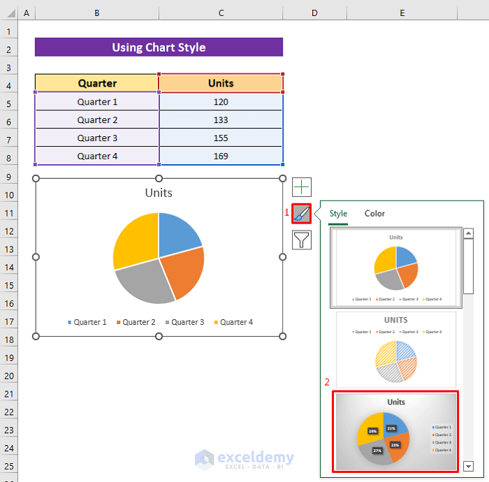
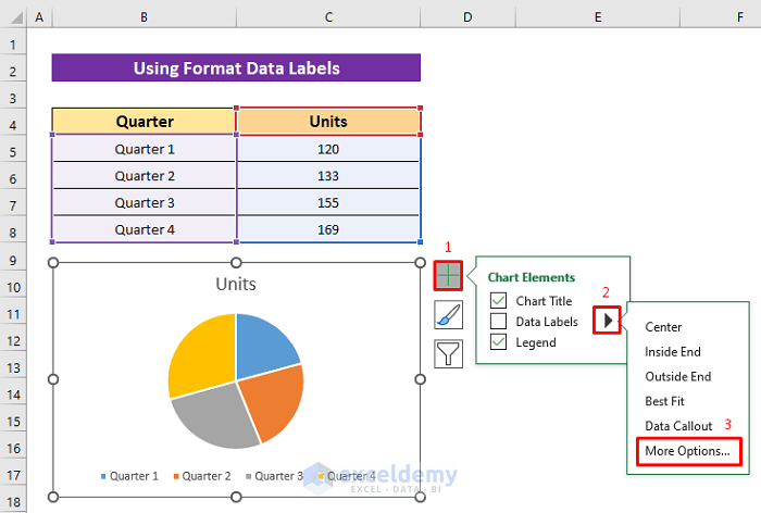
› excel-pie-chart-percentageHow to Show Percentage in Excel Pie Chart (3 Ways) Sep 08, 2022 · Another way of showing percentages in a pie chart is to use the Format Data Labels option. We can open the Format Data Labels window in the following two ways. 2.1 Using Chart Elements. To active the Format Data Labels window, follow the simple steps below. Steps: Click on the pie chart to make it active.

Data labels excel pie chart
Move data labels - support.microsoft.com Right-click the selection > Chart Elements > Data Labels arrow, and select the placement option you want. Different options are available for different chart types. For example, you can place data labels outside of the data points in a pie chart but not in a column chart. Chart.ApplyDataLabels method (Excel) | Microsoft Learn For the Chart and Series objects, True if the series has leader lines. Pass a Boolean value to enable or disable the series name for the data label. Pass a Boolean value to enable or disable the category name for the data label. Pass a Boolean value to enable or disable the value for the data label. How to display leader lines in pie chart in Excel? - ExtendOffice To display leader lines in pie chart, you just need to check an option then drag the labels out. 1. Click at the chart, and right click to select Format Data Labels from context menu. 2. In the popping Format Data Labels dialog/pane, check Show Leader Lines in the Label Options section. See screenshot:
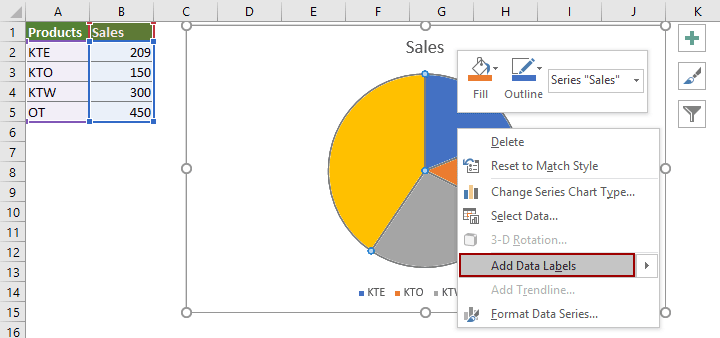
Data labels excel pie chart. Pie Chart in Excel | How to Create Pie Chart - EDUCBA Step 1: Do not select the data; rather, place a cursor outside the data and insert one PIE CHART. Go to the Insert tab and click on a PIE. Step 2: once you click on a 2-D Pie chart, it will insert the blank chart as shown in the below image. Step 3: Right-click on the chart and choose Select Data. Add or remove data labels in a chart - support.microsoft.com Click the data series or chart. To label one data point, after clicking the series, click that data point. In the upper right corner, next to the chart, click Add Chart Element > Data Labels. To change the location, click the arrow, and choose an option. If you want to show your data label inside a text bubble shape, click Data Callout. › how-to-create-excel-pie-chartsHow to Make a Pie Chart in Excel & Add Rich Data Labels to ... Sep 08, 2022 · In this article, we are going to see a detailed description of how to make a pie chart in excel. One can easily create a pie chart and add rich data labels, to one’s pie chart in Excel. So, let’s see how to effectively use a pie chart and add rich data labels to your chart, in order to present data, using a simple tennis related example. How to Make a Pie Chart with Multiple Data in Excel (2 Ways) - ExcelDemy In Pie Chart, we can also format the Data Labels with some easy steps. These are given below. Steps: First, to add Data Labels, click on the Plus sign as marked in the following picture. After that, check the box of Data Labels. At this stage, you will be able to see that all of your data has labels now.
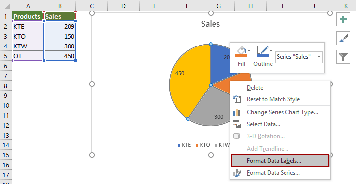
support.microsoft.com › en-us › officePresent data in a chart - support.microsoft.com To quickly identify a data series in a chart, you can add data labels to the data points of the chart. By default, the data labels are linked to values on the worksheet, and they update automatically when changes are made to these values. Add a chart title Pie Charts in Excel - How to Make with Step by Step Examples Task b: Add data labels and data callouts. Step 3: Right-click the pie chart and expand the "add data labels" option. Next, choose "add data labels" again, as shown in the following image. Step 4: The data labels are added to the chart, as shown in the following image. How to add data labels from different column in an Excel chart? Right click the data series in the chart, and select Add Data Labels > Add Data Labels from the context menu to add data labels. 2. Click any data label to select all data labels, and then click the specified data label to select it only in the chart. 3. Change the format of data labels in a chart To get there, after adding your data labels, select the data label to format, and then click Chart Elements > Data Labels > More Options. To go to the appropriate area, click one of the four icons ( Fill & Line, Effects, Size & Properties ( Layout & Properties in Outlook or Word), or Label Options) shown here.
excel - Pie Chart VBA DataLabel Formatting - Stack Overflow sub updatechartformat () with activeworkbook.sheets ("mhfa summary").chartobjects ("chart 4").activate with activechart.seriescollection (1).datalabels _ .showpercentage = true with activechart.seriescollection (1).datalabels _ .separator = "" & chr (10) & "" end with end with end with with activeworkbook.sheets ("mhfa … › how-to-create-pie-of-pieHow to Create Pie of Pie Chart in Excel? - GeeksforGeeks Jul 30, 2021 · The Pie Chart obtained for the above Sales Data is as shown below: The pie of pie chart is displayed with connector lines, the first pie is the main chart and to the right chart is the secondary chart. The above chart is not displaying labels i.e, the percentage of each product. Hence, let’s design and customize the pie of pie chart ... Edit titles or data labels in a chart - support.microsoft.com On a chart, click one time or two times on the data label that you want to link to a corresponding worksheet cell. The first click selects the data labels for the whole data series, and the second click selects the individual data label. Right-click the data label, and then click Format Data Label or Format Data Labels. Excel Pie Chart and Percentage Data Labels - YouTube In this video you will see how to create Pie chart and add to it Percentage Data Labels.Excel SuperHero book: | Int...
How to make a pie chart in Excel
Create a Pie Chart in Excel (Easy Tutorial) Create the pie chart (repeat steps 2-3). 7. Click the legend at the bottom and press Delete. 8. Select the pie chart. 9. Click the + button on the right side of the chart and click the check box next to Data Labels. 10. Click the paintbrush icon on the right side of the chart and change the color scheme of the pie chart.

PowerPoint Data Labels on Pie of Pie Charts | MrExcel Message ...
Creating Pie Chart and Adding/Formatting Data Labels (Excel) Creating Pie Chart and Adding/Formatting Data Labels (Excel)
Create a Pie Chart in Excel (Easy Tutorial)
trumpexcel.com › pie-chartHow to Make a PIE Chart in Excel (Easy Step-by-Step Guide) Creating a Pie Chart in Excel. To create a Pie chart in Excel, you need to have your data structured as shown below. The description of the pie slices should be in the left column and the data for each slice should be in the right column. Once you have the data in place, below are the steps to create a Pie chart in Excel: Select the entire dataset

How to Make Pie Chart with Labels both Inside and Outside ...
Excel Pie Chart - How to Create & Customize? (Top 5 Types) We will customize the Pie Chart in Excel by Adding Data Labels. Scenario 1: The procedure to add data labels are as follows: Click on the Pie Chart > click the ' + ' icon > check/tick the " Data Labels " checkbox in the " Chart Element " box > select the " Data Labels " right arrow > select the " Outside End " option. We get the following output.

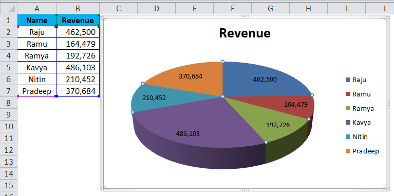
How to Create a 3D Pie Chart in Excel (with Easy Steps)
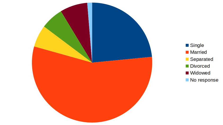
excelunlocked.com › pie-chart-in-excelPie Chart in Excel - Inserting, Formatting, Filters, Data Labels Dec 29, 2021 · The total of percentages of the data point in the pie chart would be 100% in all cases. Consequently, we can add Data Labels on the pie chart to show the numerical values of the data points. We can use Pie Charts to represent: ratio of population of male and female of a country. proportion of online/offline payment modes of a local car rental ...

Create a Dynamic Pie Chart with Dynamic Legend in Excel which ...
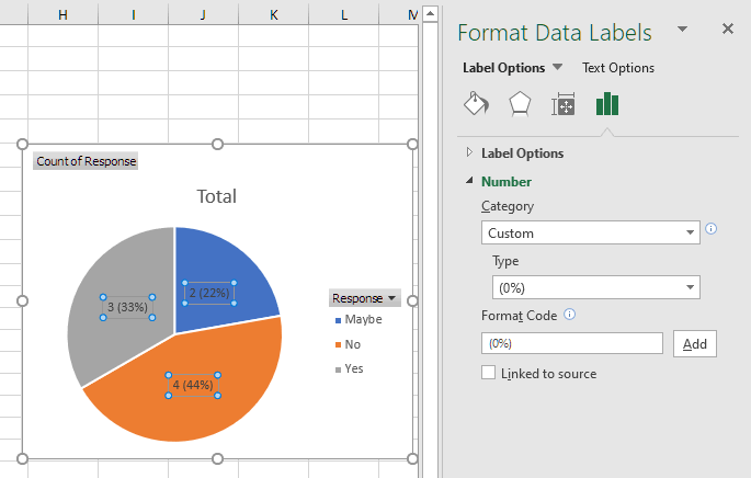
› documents › excelHow to hide zero data labels in chart in Excel? - ExtendOffice If you want to hide zero data labels in chart, please do as follow: 1. Right click at one of the data labels, and select Format Data Labels from the context menu. See screenshot: 2. In the Format Data Labels dialog, Click Number in left pane, then select Custom from the Category list box, and type #"" into the Format Code text box, and click Add button to add it to Type list box.

how to add data labels into Excel graphs — storytelling with data
How to display leader lines in pie chart in Excel? - ExtendOffice To display leader lines in pie chart, you just need to check an option then drag the labels out. 1. Click at the chart, and right click to select Format Data Labels from context menu. 2. In the popping Format Data Labels dialog/pane, check Show Leader Lines in the Label Options section. See screenshot:
:max_bytes(150000):strip_icc()/cookie-shop-revenue-58d93eb65f9b584683981556.jpg)
How to Create and Format a Pie Chart in Excel
Chart.ApplyDataLabels method (Excel) | Microsoft Learn For the Chart and Series objects, True if the series has leader lines. Pass a Boolean value to enable or disable the series name for the data label. Pass a Boolean value to enable or disable the category name for the data label. Pass a Boolean value to enable or disable the value for the data label.

Add or remove data labels in a chart
Move data labels - support.microsoft.com Right-click the selection > Chart Elements > Data Labels arrow, and select the placement option you want. Different options are available for different chart types. For example, you can place data labels outside of the data points in a pie chart but not in a column chart.

EXCEL Charts: Column, Bar, Pie and Line

How to make doughnut chart with outside end labels - Simple ...
How-to Make a WSJ Excel Pie Chart with Labels Both Inside and ...
Pie Chart in Excel | How to Create Pie Chart | Step-by-Step ...

Pie Chart – Excel Tutorial

Change the format of data labels in a chart

Creating Pie Chart and Adding/Formatting Data Labels (Excel)

Change color of data label placed, using the 'best fit ...

How to Create a Pie Chart in Excel | Smartsheet

How to Make a Pie Chart in Excel - All Things How
KB209780: Data labels overlap when exporting a pie graph in a ...
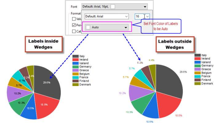
Help Online - Quick Help - FAQ-1019 How to customize the font ...

How to Change Excel Chart Data Labels to Custom Values?

Office: Display Data Labels in a Pie Chart
How to Show Pie Chart Data Labels in Percentage in Excel

Change the format of data labels in a chart
Excel custom pie chart labels - Microsoft Community

How to make a pie chart in Excel

Add data labels and callouts to charts in Excel 365 ...
How to Show Pie Chart Data Labels in Percentage in Excel

How to Make Pie Chart with Labels both Inside and Outside ...

How to Make a Pie Chart in Excel - All Things How

Custom data labels in a chart
How to show percentage in pie chart in Excel?
How to show percentage in pie chart in Excel?

How to show percentages on three different charts in Excel ...

How to fix wrapped data labels in a pie chart | Sage Intelligence
Is there a way to prevent pie chart data labels from ...

Change the format of data labels in a chart
5 Common Data Visualization Mistakes to Avoid - Hoji

How-to Add Label Leader Lines to an Excel Pie Chart - Excel ...
Post a Comment for "40 data labels excel pie chart"