42 excel chart change labels

How to Change Font Size of Data Labels in Excel - ExcelDemy Fourthly, select the whole graph and click on the Chart Elements option and go to the Data Labels. After that, you will get the result like the below image. Next, select the data chart and go to the Home tab. Then, choose the font size accordingly. Finally, the following result will come up on your screen. 2. Chart.ApplyDataLabels method (Excel) | Microsoft Docs The type of data label to apply. True to show the legend key next to the point. The default value is False. True if the object automatically generates appropriate text based on content. For the Chart and Series objects, True if the series has leader lines. Pass a Boolean value to enable or disable the series name for the data label.

Format Chart Axis in Excel - Axis Options However, In this blog, we will be working with Axis options, Tick marks, Labels, Number > Axis options> Axis options> Format Axis Pane. Axis Options: Axis Options There are multiple options So we will perform one by one. Changing Maximum and Minimum Bounds The first option is to adjust the maximum and minimum bounds for the axis.

Excel chart change labels

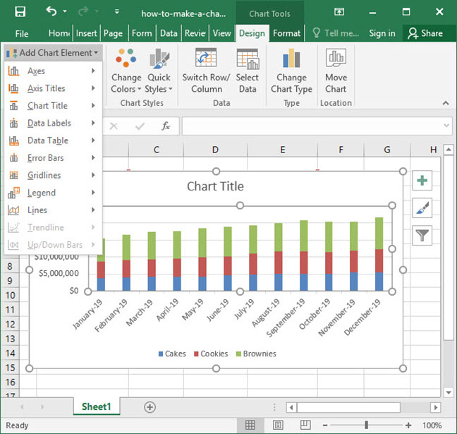
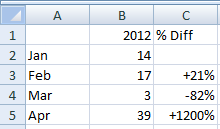
How to Change the Y Axis in Excel - Alphr To change the axis label's position, go to the "Labels" section. Click the dropdown next to "Label Position," then make your selection. Changing the Display of Axes in Excel All About Chart Elements in Excel - Add, Delete, Change - Excel Unlocked By default, Excel writes the text string "Chart Title" at the place of the chart title. We can rename the chart title by double-clicking on it. i.e "Monthly Sales" We can also change the position of the chart title by simply dragging it using the cursor. Download Above Image to Your Desktop >>>> Download Chart Data Labels How to Create a Bubble Chart in Excel with Labels (4 Easy Ways) Next, click on Data Labels >> select More Data Label Options. Now, the Format Data Labels toolbox will appear. Next, from Label Options select Above as Label Position. Then, select Value From Cells in Label Contains. After that, the Data Label Range box will open. Next, select Cell range B5:B9 in the Select Data Label Range box. Now, press OK.

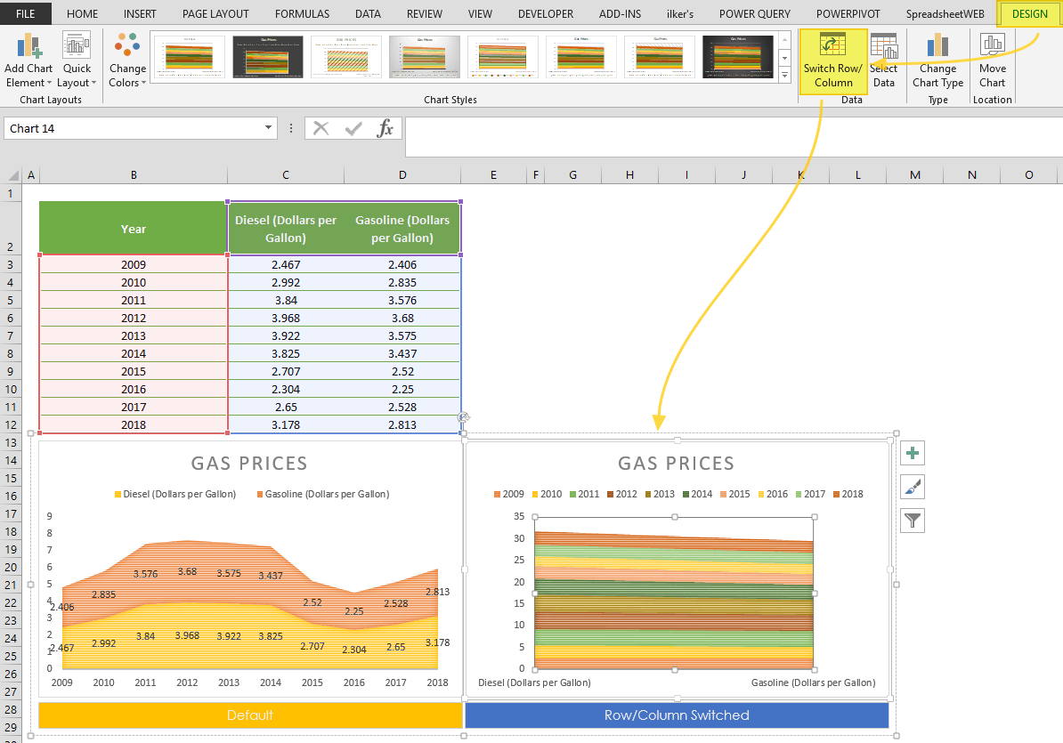
Excel chart change labels. How to format axis labels individually in Excel - SpreadsheetWeb Double-click on the axis you want to format. Double-clicking opens the right panel where you can format your axis. Open the Axis Options section if it isn't active. You can find the number formatting selection under Number section. Select Custom item in the Category list. Type your code into the Format Code box and click Add button. How to Change Data Labels in Excel (with Easy Steps) Go to the chart. Double click on any of the bars. All the bars are in the editable mode now. Press the right button of the mouse. Choose Add Data Labels option from the Context Menu. Look at the chart. We can see the value of each bar is shown at the top of each bar. 📌 Step 3: Change Data Labels How to change dot label(when I hover mouse on that dot) of - Microsoft ... How to change dot label (when I hover mouse on that dot) of scatter plot. Hello all, I have few queries: 1. Can I edit the text when I hover mouse on dot of scatter plot (chart) 2. Can I use url to redirect to different site. 3. Can I use display image if I hover mouse on the dot. Excel: How to Create a Bubble Chart with Labels - Statology Step 2: Create the Bubble Chart. Next, highlight the cells in the range B2:D11. Then click the Insert tab along the top ribbon and then click the Bubble Chart option within the Charts group: The x-axis displays the points, the y-axis displays the assists, and the size of each bubble represents the rebounds.

How to Add Axis Titles in a Microsoft Excel Chart Select your chart and then head to the Chart Design tab that displays. Click the Add Chart Element drop-down arrow and move your cursor to Axis Titles. In the pop-out menu, select "Primary Horizontal," "Primary Vertical," or both. If you're using Excel on Windows, you can also use the Chart Elements icon on the right of the chart. Chart data labels and CAGR arrows - UpSlide Help & Support On the dropdown select Labels to open the label editor Under Select the Series dropdown choose the series you want to add labels to (this step is only necessary when your chart has multiple series present) Use the range selector to choose the cell contents you want to display, press enter to return to the label editor How to Format Data Labels in Excel (with Easy Steps) I hope you enjoy this article and find it interesting. Table of Contents hide. Download Practice Workbook. Step-by-Step Procedure to Format Data Labels in Excel. Step 1: Create Chart. Step 2: Add Data Labels to Chart. Step 3: Modify Fill and Line of Data Labels. Step 4: Change Effects to Format Data Labels. How to make shading on Excel chart and move x axis labels to the bottom ... In the Change Chart Type dialog, change the chart type for the new series to Stacked Area. Change the color from whatever Excel decides to yellow. Finally, remove the new series form the legend. See the attached version.

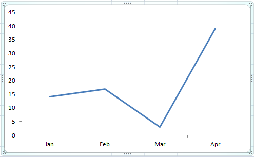
change Excel chart label position Archives - Data Cornering Tag: change Excel chart label position. Excel. How to move Excel chart axis labels to the bottom or top. by Janis Sturis July 25, 2022 Comments 0. Categories. Custom Chart Data Labels In Excel With Formulas Follow the steps below to create the custom data labels. Select the chart label you want to change. In the formula-bar hit = (equals), select the cell reference containing your chart label's data. In this case, the first label is in cell E2. Finally, repeat for all your chart laebls. Excel charts: Labels on X-axis start at the wrong value If this does not work, you can also select the x-axis in the following way; assuming you are able to adjust the y-axis as mentioned in your comment. Select the y-axis -> right click -> Format Axis.... Inside Format Axis you need to select Axis Options and select Horizontal (Value) Axis: Share. edited Jul 18 at 18:30. answered Jul 18 at 9:17. karl. How to add text labels on Excel scatter chart axis Select recently added labels and press Ctrl + 1 to edit them. Add custom data labels from the column "X axis labels". Use "Values from Cells" like in this other post and remove values related to the actual dummy series. Change the label position below data points. Hide dummy data series markers by switching marker options to none. 5.

How To Make a Chart In Excel | Deskbright

Excel Area Chart Data Label & Position - ExcelDemy You can use it to draw attention to the change over time and show the total value across a trend. Excel allows us to insert both 2-D and 3-D area charts. There are three types of area charts available in excel. An area chart displays the change of values over time. A Stacked Area Chart shows the change in the contribution of each value over time.

Change Series Name Excel Mac

How to Edit Pie Chart in Excel (All Possible Modifications) Just like the chart title, you can also change the position of data labels in a pie chart. Follow the steps below to do this. 👇 Steps: Firstly, click on the chart area. Following, click on the Chart Elements icon. Subsequently, click on the rightward arrow situated on the right side of the Data Labels option.

Excel Course: Inserting Graphs

How to add data labels in excel to graph or chart (Step-by-Step) 1. Select a data series or a graph. After picking the series, click the data point you want to label. 2. Click Add Chart Element Chart Elements button > Data Labels in the upper right corner, close to the chart. 3. Click the arrow and select an option to modify the location. 4.

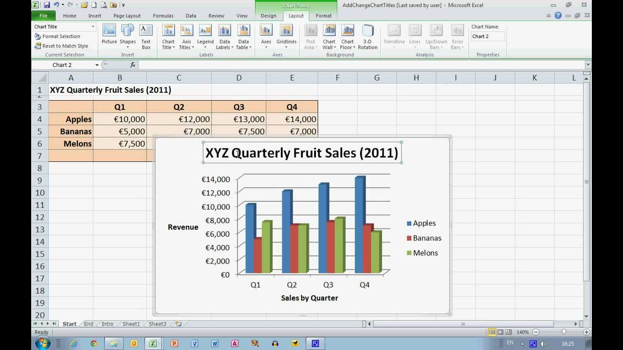
How To... Add and Change Chart Titles in Excel 2010 - YouTube

How to Create and Customize a Waterfall Chart in Microsoft Excel Select the chart and use the buttons on the right (Excel on Windows) to adjust Chart Elements like labels and the legend, or Chart Styles to pick a theme or color scheme. Select the chart and go to the Chart Design tab.

Improve your X Y Scatter Chart with custom data labels

How do I add a label to a chart in Excel? - Foley for Senate Click on your chart. Click the Layout tab under Chart Tools. Click Axis Titles in the Labels group. Point to Primary Horizontal Axis Title and select Title Below Axis. How do you change the horizontal axis labels in Excel? To change the format of numbers on the value axis: Right-click the value axis labels you want to format. Click Format Axis.

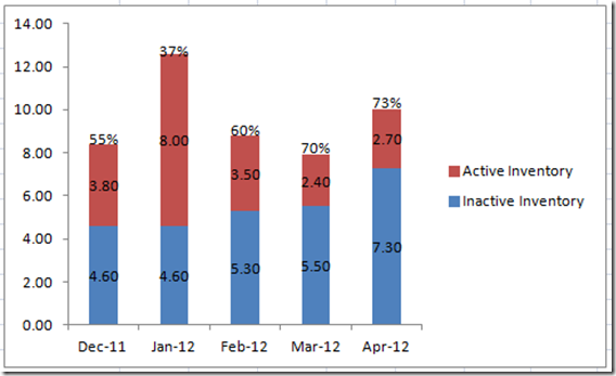
How-to Put Percentage Labels on Top of a Stacked Column Chart - Excel Dashboard Templates

Modifying Axis Scale Labels (Microsoft Excel) Follow these steps: Create your chart as you normally would. Double-click the axis you want to scale. You should see the Format Axis dialog box. (If double-clicking doesn't work, right-click the axis and choose Format Axis from the resulting Context menu.) Make sure the Number tab is displayed. (See Figure 1.) Figure 1.

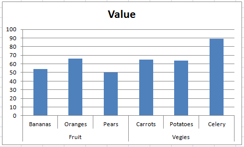
Fixing Your Excel Chart When the Multi-Level Category Label Option is Missing. - Excel Dashboard ...

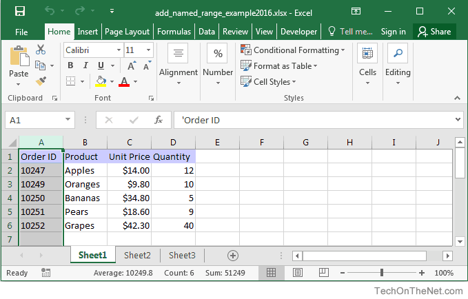
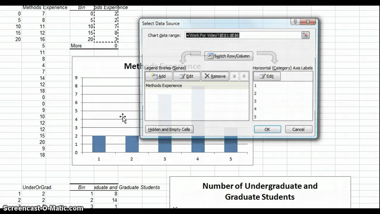
Use defined names to automatically update a chart range - Office On the Insert menu, click Chart to start the Chart Wizard. Click a chart type, and then click Next. Click the Series tab. In the Series list, click Sales. In the Category (X) axis labels box, replace the cell reference with the defined name Date. For example, the formula might be similar to the following: =Sheet1!Date

Area Chart in Excel

How to Add Labels to Scatterplot Points in Excel - Statology Step 3: Add Labels to Points Next, click anywhere on the chart until a green plus (+) sign appears in the top right corner. Then click Data Labels, then click More Options… In the Format Data Labels window that appears on the right of the screen, uncheck the box next to Y Value and check the box next to Value From Cells.

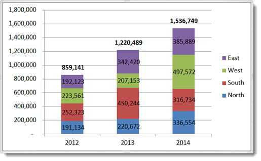
How to Show Percentages in Stacked Bar and Column Charts in Excel

Change axis labels in a chart - Microsoft Support

Custom Data Labels with Colors and Symbols in Excel Charts - [How To] - PakAccountants.com ...

How to Apply a Filter to a Chart in Microsoft Excel Go to the Home tab, click the Sort & Filter drop-down arrow in the ribbon, and choose "Filter.". Click the arrow at the top of the column for the chart data you want to filter. Use the Filter section of the pop-up box to filter by color, condition, or value. When you finish, click "Apply Filter" or check the box for Auto Apply to see ...

How-to Add Custom Labels that Dynamically Change in Excel Charts - Excel Dashboard Templates

How to Print Labels from Excel - Lifewire Select Mailings > Write & Insert Fields > Update Labels . Once you have the Excel spreadsheet and the Word document set up, you can merge the information and print your labels. Click Finish & Merge in the Finish group on the Mailings tab. Click Edit Individual Documents to preview how your printed labels will appear. Select All > OK .

How to Make Charts and Graphs in Excel | Smartsheet

How to Create a Bubble Chart in Excel with Labels (4 Easy Ways) Next, click on Data Labels >> select More Data Label Options. Now, the Format Data Labels toolbox will appear. Next, from Label Options select Above as Label Position. Then, select Value From Cells in Label Contains. After that, the Data Label Range box will open. Next, select Cell range B5:B9 in the Select Data Label Range box. Now, press OK.

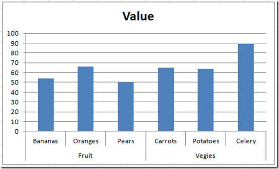
Excel Dashboard Templates Fixing Your Excel Chart When the Multi-Level Category Label Option is ...

All About Chart Elements in Excel - Add, Delete, Change - Excel Unlocked By default, Excel writes the text string "Chart Title" at the place of the chart title. We can rename the chart title by double-clicking on it. i.e "Monthly Sales" We can also change the position of the chart title by simply dragging it using the cursor. Download Above Image to Your Desktop >>>> Download Chart Data Labels